Congratulations!
You just learned something with reinforcement learning (RL): click on the circles!The basic concept of RL is simple: an agent is in a state and may perform different actions, which lead to new states. The actions are rewarded or punished (a punishment may also be called “negative reward”). Based on the received rewards, the agent learns to perform the desired actions.
Wait, but how do these terms map on the game with the squares and circles? Scroll down to find out!
In this case, there were two possible "actions" in each state: clicking on the square, or clicking on the circle, which gave a reward in the case of the circle, and a punishment in the square-case.
So the state could be seen as the input, the agent as the algorithm, and the action as the output.

For the purpose of this introduction, I will use the following notation. This will only be relevant for some Detail Chapters, so you don’t need it to understand the main lessons.
s := state
a := action
r := reward
p(x|y) := probability of x, under the condition y
Example: p(s’,r|s,a) is the probability of transition to state s’ with reward r, when action a is taken in state s.
In other words, if you’re in state s and execute action a, what’s the probability of landing in state s’ with reward r? This probability is represented by p(s’,r|s,a).
humans are Reinforcement Learners
(and because it was an easy exercise). Evolution came up with this concept and it worked extremely well, so well in fact that nowadays almost all animals have it.Reinforcement learning in Animals
Since “reinforcement learning” is a pretty broad term that includes lots of different algorithms, it is quite imprecise to say that animals have “it”.
It is quite clear that animals (including humans) use some form of RL, and also quite clear that they don’t use all RL algorithms that some random computer scientist ever came up with.
Which forms of RL animals use exactly is still being debated and not conclusively established, but let’s have a look at what science has uncovered!
One paradigm of RL that seems to play a big role in animals is called “Temporal Difference Learning”, or short: TD learning. Ever heard of the neurotransmitter “dopamine”, which is often colloquially called the “pleasure hormone” or the like? It is true that dopamine is, among other things, related to pleasure (reward!). But it seems that this is not the whole story; it is now believed that dopamine represents the anticipation of reward, or more precisely, it represents the prediction error of the reward. What the hell does that mean?
It is actually quite simple: the brain has expectations about the amount of reward a certain action will bring. The difference between this predicted reward and the actual outcome is called the prediction error. If there’s more reward than expected, certain neurons show increased activity, and more dopamine than usual is emitted, which leads to a better prediction next time - learning has occured. This means describing dopamine as a simple reward neurotransmitter would be wrong - there is no dopamine reaction even in cases of very high reward, as long as the reward was already anticipated.
(Actually, it is not the difference in reward that’s computed, but rather the difference in state utilities (between expected utility and newly computed utility) - more on that later!)
Since it works so well in nature, computer science has adopted it as a Machine Learning (ML) technique, with huge success. As a consequence, RL is now a hot topic within the fields of computer science and psychology, and progress in either context can often be applied to the other field. This means new algorithms or insights that stem from computer science often help to deepen our understanding of RL in animals. On the other hand, the more we find out about how RL is implemented in the brain, the closer we get to building artificial general intelligence (AGI), an AI that is on par with humans in cognitive abilities and might even surpass them soon thereafter.
Is that a goal we should work on? People disagree on this, but Google's DeepMind certainly thinks so.
But what if, by clicking on a square 20x in a row (getting punished each time), you would have been redirected to a hidden page that gives you a 20€ Amazon voucher? Obviously, this would have been worth the pain of getting a red-screen-punishment 20 times.
So maybe, you should have tried clicking on the square 20 times. But what if the threshold was at 30? Or 40? When should you stop smashing that square button like a mad person, performing the same action over and over again, expecting a different result?
The trade-off between exploration and exploitation
is the first one. When you learn something new, you first want to try out many different actions to find out which ones are the most rewarding (exploration). You are not satisfied with the first action that yields a positive reward, because there might be even better actions! But at some point, you want to use what you’ve learned so far and choose the actions that gave you the highest reward in the past (exploitation). The question is: how much should you explore, and when should you start exploiting your knowledge? Should you stop exploring completely at some point or still try out new things once in a while? If you don’t know the general answer, it’s because there is none. The right approach depends on the circumstances, and is in many cases simply not known. In most cases it's probably a good idea to start with a lot of exploration, and gradually shift the strategy towards more exploitation, only maintaining a very small amount of exploration after a lot of learning has already taken place.Selecting actions in a way that always exploits current knowledge is called greedy. “Greedy action selection always exploits current knowledge to maximize immediate
reward; it spends no time at all sampling apparently inferior actions to see if they might really be better.” [1]
Of course with this method, the algorithm can’t learn very well. A simple way to exploit knowledge a lot, but which also guarantees we will also discover the best actions in the long run, is the ε-greedy method: it is greedy most of the time, but with a small probability ε, it selects a random action. For example, ε-greedy action selection with ε = 0.1 selects the best action, according to our current knowledge, 90% of the time, and in 10% of the cases it chooses a random action.
So what’s a good ε value? This depends on the circumstances, but here are some reflections. An ε value of 0 (meaning a greedy method) performs better in the short run, but might perform worse in the long run (by getting stuck in local maxima), because it never explores seemingly bad options. A big ε finds better actions quickly, but keeps on performing random (suboptimal) actions with the same big ε probability. A small ε on the other hand improves more slowly, because it doesn’t try out new things that much, but eventually it will surpass the other two because it finds the optimal actions and only rarely chooses a random action, selecting the best actions almost always after a lot of training. [1]
As a compromise, one can use a shrinking ε value that starts out big and approaches 0 over time. In a static environment, this algorithm would learn quickly in the beginning, and transition to exploiting this knowledge more and more.
This being said, an ε value that never goes under a certain threshold is still better suited for a changing environment where the optimal actions change over time.
[1] R Sutton, A. Barto. 2017. Reinforcement Learning: An Introduction ****Complete Draft**** p. 21-22
The latter seems sensible, until you realize that the future reward might be infinite and you can’t calculate the best action anymore.
In practice, most algorithms strike a balance here, and count reward that’s far away in the future much less than the reward of the next action. This is called
discounting
The discount rate is written as gamma:
γ := discount rate
t := time step
Example: Rt = rt + γ*rt+1 + γ²*rt+2 ...
In other words, if we see the future as different paths and the actions are the choices we make at the forks that lie ahead, we always want to take the fork that gives us access to the path that contains the most reward points, IF we decide optimally at all following forks.
This sum of potential future rewards is called "value" or
utility
Here, I will use the term "utility", because it is less ambiguous than "value".Above, I said "ideally", because usually we don't know for certain which action has the highest potential for future reward - but we might have an expectation. This expectation is called
expected utility
state
contains complete information about the environment we’re in, but most of the time we can’t fully know everything that’s going on. So more realistically, the state contains all the information that we know and that we also want to use for our decisions. For example in a chess game, it would describe the position of all the pieces, but for a self-driving car, the state would not contain all the positions of every single atom in the world, it would consist of all the sensory input, which is of course just an approximation of the real world.The equation that describes the optimal actions with regard to their future reward potential is known as the “Bellman optimality equation”.
Let’s define the function that gives us the utility u (the sum of future rewards) of a state s. The utility would of course depend on the actions that the agent takes in the future. The book of rules that guides the behaviour of an agent is called a policy, denoted as 𝜋.
Then the function would look like this
u𝜋(s)
Meaning: the utility u of a state s when following the policy 𝜋.
Earlier I said we want to take the fork that gives us access to the path with the most utility, under the premise that we decide optimally at all following forks. The function that returns the utility of a state under an optimal policy 𝜋* (meaning the agents makes optimal decisions) is written like this
u*(s)
Now, if we want to know which path to take, we’d have to look up where the paths lead and calculate the utility of all the states that we can reach ( u*(s1), u*(s2), u*(s3), …).
It gets even easier when we use a function that gives us the utility of a certain action that we can choose when we are in a specific state. In order to not confuse this function with the other function, let’s denote the utility function as q this time.
So let’s define the function that gives us the utility of an action a, when we’re in state s, under an optimal policy, as
q*(s, a)
This function returns the utility of an action that we decide on in a specific state (the same action might yield different results in different states).
Okay, so we defined a function, but how does the term for computing the utility actually look like?
Or, when expressed in regard to a state-action-pair:
This is the Bellman optimality equation.
u*(s) is interpreted as such:
Of the available actions in state s, choose the one with the maximum sum that is comprised of the probability of a reward, times the reward plus the utility of the next state. The utility of the next state is discounted by the discount rate γ.
As you can see, it is recursive: u*(s) contains u*(s’), where s’ is the next state. This means writing the whole equation down for an actual RL problem would be infeasible for a human, but it’s standard practice for a computer, and makes this a part of dynamic programming.
This is the theoretically ideal solution for an environment of which the dynamics are known. So did we already “solve” reinforcement learning for environments where we have complete information? Unfortunately, not at all. As you might already suspect, since it is recursive, the Bellman optimality equation takes unfathomable amounts of computing power and memory in complex environments, which makes it infeasible for almost all real world applications. Additionally, the most interesting problems which we want so solve with ML often have incomplete information, meaning the dynamics of the environment are not fully known. Still, the Bellman optimality equation is important groundwork, and many RL algorithms build on it by trying to approximate its solution [1].
[1] https://www.tu-chemnitz.de/informatik/KI/scripts/ws0910/ml09_3.pdf - p.25/slide 48
Think of an autonomous car: the number of different speed-states isn’t that high. Even if you don’t round, and the speed parameter has a precision of 3 decimal places (like 34.585 km/h), there are only about 150’000 different states - that’s nothing for a computer. The car could simply learn the optimal action for each of the 150’000 states, like “break with a force of 5.0” at the speed of 148.999 km/h, or “speed up with a force of 3.1” at the speed of 5.122 km/h, right?
Except of course the parameter of speed alone is useless, the decision to break or speed up can’t be made solely by knowing how fast the car is going. You need to consider a lot of parameters in combination, like distance to car in front, distance to car behind, steepness of the curve, probability of pedestrians jumping on the street etc. But if you have 150’000 different possible values for each parameter, and just 10 parameters (you’d probably have many more), this suddenly creates 5.76650390625×1051 distinct states - that’s about 6 sexdecillion states. Even if you rounded all parameters to only 150 different values per parameter, you’d still have around 1021 states - a one-petabyte hard drive only has 1015 bytes, so you would need at least 1 million of them just to save all the possible states, and then you’d still need to figure out a policy to navigate through that state-space.
function approximation
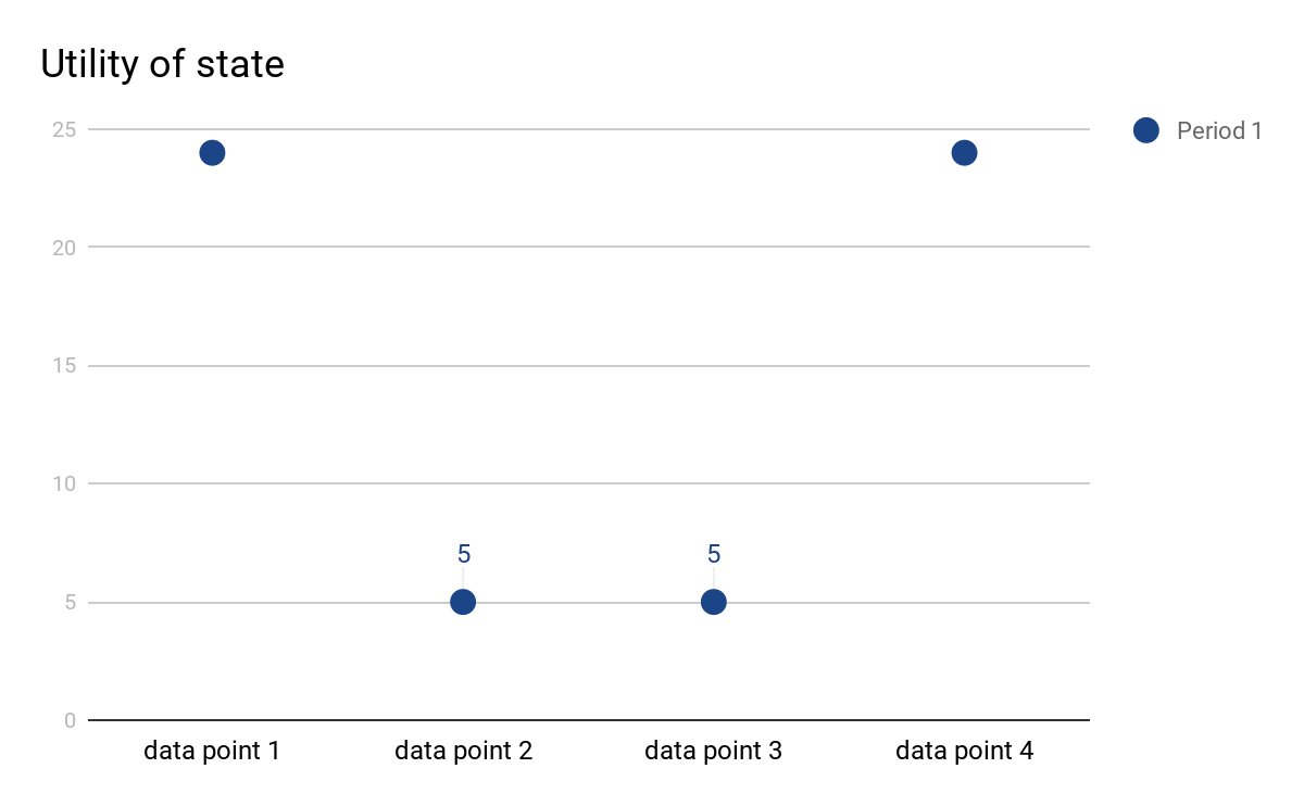
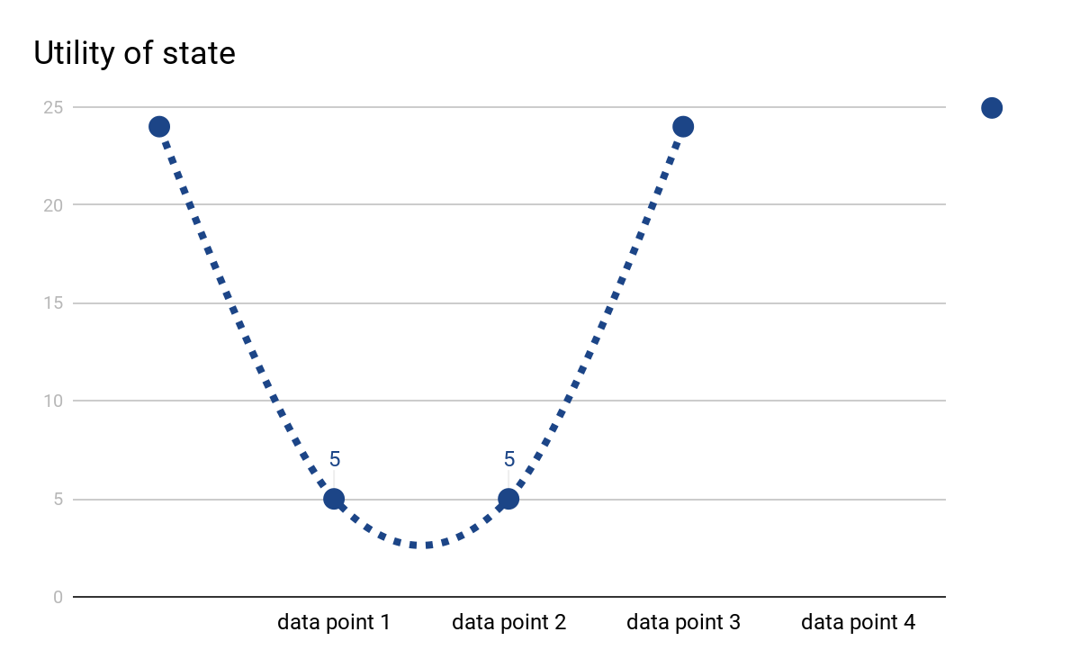
Imagine you have a function where you put in a state, and it gives back to you the true utility of that state. You could use it to calculate the utility of the next possible states that you can reach from the state you’re in, and you would then choose the action that brings you to the state with the highest utility. That function exists somewhere, even if we don’t know how it looks, and if we assume some regularity (meaning that there is a kind of pattern in the relationship between states and utility), knowing only a few points of the graph (tuples of parameters and utility) should tell us something about the rest of the graph. Of course, the more points we know, the better we can approximate the function.Which function describes all 4 data points?

A parabola!

So based on the data we got, we might assume that our utility function is something like
Utility(state) = state2
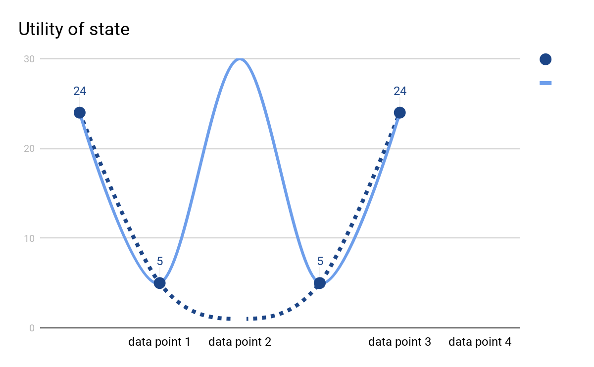
Based on that, we can calculate the utilities of states which we never encountered in our training (and therefore don’t know the long-term expected reward) and decide how we should act in an unknown situation! Of course, with so little data, our approximation is likely to be quite erroneous. Have a look at how the same set of points can be described by different functions:

For example, if the x-axis was describing a car’s position on a 3 lane highway, we might have had good experiences with driving on the right and driving on the left. The data points in between have low utility, because they describe the position between the left/right lane and the center lane - driving between lanes is not rewarded highly! But we don’t realize that the actual function has a spike in the middle, because driving on the middle lane is also okay. This example was of course simplified to the extreme; in reality, the function has a lot more than two dimensions, about a million or more, and it’s much more difficult to find a function that describes the available data points. One particular form of function approximation that you have probably heard of are “Neural Networks”. The combination of RL and NN is extremely powerful and has yielded results like the groundbreaking “Alpha Go” by Google. Just remember that NNs themselves are not goal-oriented, that’s where RL comes into play! And although NNs are very popular, they are not the only powerful form of function approximation.
the end
And that’s it! You now know about the key concepts and problems in reinforcement learning. Congratulations!For some hands on experience, I created a Jupyter Notebook that presents and explains an RL-algorithm: policy iteration. You can execute the code to solve an actual problem and even modify it if you want to! To initialize the notebook with binder, klick on this button:
You may view and download all the files on GitHub.
If you would like to learn a lot more from the pioneers of reinforcement learning themselves, go check out this freely available and extraordinarily well written book by Richard Sutton and Andrew Barto.
Or you could sign up for a MOOC if you prefer a university-style seminar. There are many different MOOCs on the topic out there. For folks with a degree in computer science (or similar), I can recommend this course by Georgia Tech.
Square and circle puzzle created by Andreas Plewnia for this introduction.